My data pipeline journey with Environ

Introducing Environ

Background & Motivation

In collaboration with Environ, we developed an IoT solution that streams data from solar panels, batteries, energy production and consumption, and more to the cloud.

Defining the Task

Our goal was to answer a key question: ‘How much did I actually pay for my energy at a specific time?’

With access to all the necessary data - such as time-specific kilowatt-hour prices from a given energy provider - this task was not only feasible but also highly valuable for our users.

Where We Began

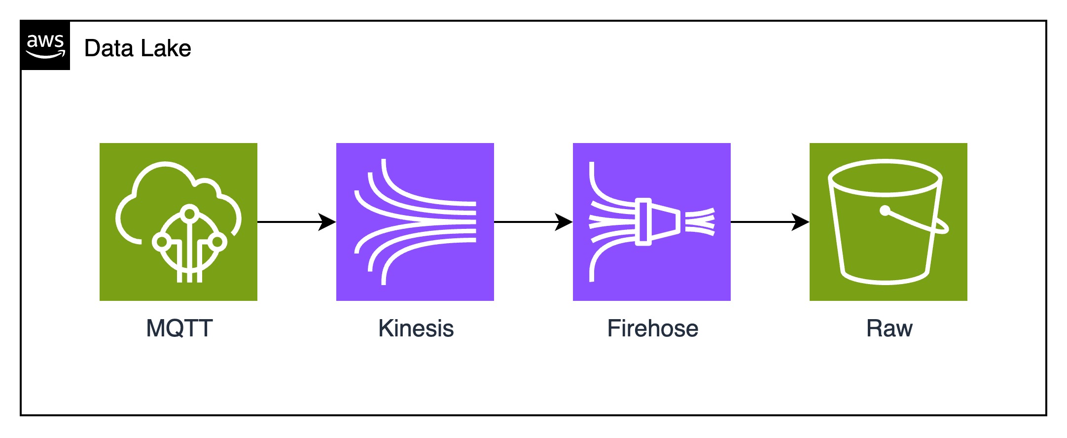
Before diving into the solution, we first needed to evaluate our data sources. We were already receiving a high volume of events per device, which gave us a solid foundation to work from. However, we quickly realized that the original data wasn’t being persisted—most of it was processed in real-time and then discarded. To address this, we set up a Data Lake and began streaming raw events into it using Amazon Kinesis.

Here you can find an AWS whitepaper

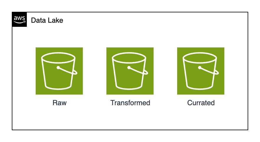
Based on this Whitepaper, this is the structure: A data lake can be broadly categorized across four distinct buckets:

• Raw – Original data collected from sources, stored as it is. This can include structured, semi-structured, or unstructured files like JSON, CSV, XML, text, or images.
• Transformed – Raw data is cleaned, enriched and converted into efficient formats (like Parquet) for better performance and lower costs.
• Curated – Transformed data is further refined and combined with other data to gain deeper insights. It’s optimized for analytics, reporting, and use in tools like Amazon Athena, Redshift Spectrum, or Amazon Redshift.

That’s the Buckets we’ve created

That’s how the ingestion process looks like

Once the Data Was In

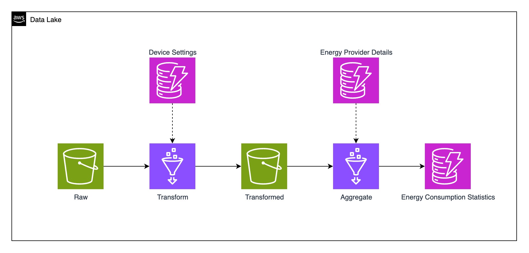
After collecting the data, we were creating the ETL-Process, which takes the raw data, enriches it with data we need and then created aggregations for querying.

Our ETL-Pipeline

We scheduled the pipeline to run every hour using an AWS Step Function. The transformation job processes the raw events—referred to as measurements—and enriches them with the energy provider ID, which is configurable on the device but not included in the event payload. Next, the aggregation job takes these transformed events, retrieves additional energy provider details, and calculates the corresponding energy costs. Finally, the results are grouped into time windows and stored in DynamoDB for efficient access.

Incoming events

Those events are simplified, they contain much more information, due to simplicity I also change the timestamps to be “hourly”.

{
  "device_id": "01234ABCD",
  "timestamp": "2025-08-01T00:00:00",
  "daily_import_energy": 0
}
{
  "device_id": "01234ABCD",
  "timestamp": "2025-08-01T01:00:00",
  "daily_import_energy": 1000
}
{
  "device_id": "01234ABCD",
  "timestamp": "2025-08-01T02:00:00",
  "daily_import_energy": 2000
}

Incoming events after transformation

Now we enrich the events with the energy provider ID, which is configured in a dynamo db table.

{
  "device_id": "01234ABCD",
  "energy_provider_id": "567EFG",
  "timestamp": "2025-08-01T00:00:00",
  "daily_import_energy": 0
}
{
  "device_id": "01234ABCD",
  "energy_provider_id": "567EFG",
  "timestamp": "2025-08-01T01:00:00",
  "daily_import_energy": 1000
}
{
  "device_id": "01234ABCD",
  "energy_provider_id": "567EFG",
  "timestamp": "2025-08-01T02:00:00",
  "daily_import_energy": 2000
}

Transforming the Data: Aggregation

In the aggregation job we now have the most complex logic, first of all we create so-called “windows”.

In our calculation those windows are 1 hour long, additionally we simultaneously calculate the consumption which is max(daily_import_energy) - min(daily_import_energy).

What is daily_import_energy?

This is a value which is rested every day at 00:00 and represents the energy which was imported by an energy provider (basically bought electricity).

{
  "device_id": "01234ABCD",
  "energy_provider_id": "567EFG",
  "consumption": 1000,
  "window": {
    "start": "2025-08-01T00:00:00",
    "end": "2025-08-01T01:00:00"
  }
}
{
  "device_id": "01234ABCD",
  "energy_provider_id": "567EFG",
  "consumption": 1000,
  "window": {
    "start": "2025-08-01T01:00:00",
    "end": "2025-08-01T02:00:00"
  }
}

Since we now have the energy consumption for every timeframe, plus the information from which provider we bought it, we simply have to look up the prices in our energy price history database.

We know checking the database, that the provider with the ID 567EFG charges 20ct/kWh.

Now we just need to add this to our calculation, add some taxes and voilà - we are done.

{
  "device_id": "01234ABCD",
  "energy_provider_id": "567EFG",
  "consumption": 1000,
  "consumption_cents": 20,
  "tarrifs": 12.948,  // + 4.10ct = Stromsteuer (2.05ct/kWh)
                      // + 1.632ct = Offshore-Netzumlage (0.816ct/kWh)
                      // + 3.116ct Umlage nach Paragraph 19 (1.558ct/kWh),
                      // + 4.10ct KWK-Umlage (2.05ct/kWh),
  "net_total_with_tariffs_and_fees": 32.948, // consumption_cents + tarrifs
  "taxes": 6.26012,   // 19% off net_total_with_tariffs_and_fees
  "total": 39.20812,  // net_total_with_tariffs_and_fees + taxes
  "window": {
    "start": "2025-08-01T00:00:00",
    "end": "2025-08-01T01:00:00"
  }
}
{
  "device_id": "01234ABCD",
  "energy_provider_id": "567EFG",
  "consumption": 1000,
  "consumption_cents": 20,
  "tarrifs": 12.948,  // + 4.10ct = Stromsteuer (2.05ct/kWh)
                      // + 1.632ct = Offshore-Netzumlage (0.816ct/kWh)
                      // + 3.116ct Umlage nach Paragraph 19 (1.558ct/kWh),
                      // + 4.10ct KWK-Umlage (2.05ct/kWh),
  "net_total_with_tariffs_and_fees": 32.948, // consumption_cents + tarrifs
  "taxes": 6.26012,   // 19% off net_total_with_tariffs_and_fees
  "total": 39.20812,  // net_total_with_tariffs_and_fees + taxes
  "window": {
    "start": "2025-08-01T01:00:00",
    "end": "2025-08-01T02:00:00"
  }
}

But before we store the data, we added some more aggregations, based on week, month and year since this was requested in the feature.

The last step in this process is to store this information in a format which is easy to access, we’ve gone for dynamo db here.

{
  "PK": "DEVICE#0123ABCD",
  "SK": "DURATION#1 hour#START_TIME#2025-08-01 00:00:00",
  "window": {
    "start": "2025-08-01T00:00:00",
    "end": "2025-08-01T01:00:00"
  },
  "consumption": 1000,
  "consumption_cents": 20,
  "tarrifs": 12.948,  
  "net_total_with_tariffs_and_fees": 32.948,
  "taxes": 6.26012,
  "total": 39.20812,
}
{
  "PK": "DEVICE#0123ABCD",
  "SK": "DURATION#1 day#START_TIME#2025-08-01 00:00:00",
  "window": {
    "start": "2025-08-01T00:00:00",
    "end": "2025-08-02T00:00:00"
  },
  "consumption": 2000,
  "consumption_cents": 40,
  "tarrifs": 25.896,
  "net_total_with_tariffs_and_fees": 65.896,
  "taxes": 12.52024,
  "total": 79.41624,
}
{
  "PK": "DEVICE#0123ABCD",
  "SK": "DURATION#1 month#START_TIME#2025-08-01 00:00:00",
  "window": {
    "start": "2025-08-01T00:00:00",
    "end": "2025-09-01T00:00:00",
  },
  ...
}
{
  "PK": "DEVICE#0123ABCD",
  "SK": "DURATION#1 year#START_TIME#2025-01-01 00:00:00",
  "window": {
    "start": "2025-01-01T00:00:00",
    "end": "2026-01-01T00:00:00",
  },
  ...
}

Building the API

Before we could finish the task we had to create and endpoint in our API so it can be requested from the Envi-IQ App.

envi-iq.api/v1/devices/0123ABCD/energy-consumption-prices/hour/2025-08-01 00

{
  "consumption": 1000,
  "consumptionCents": 20,
  "tarrifs": 12.95,  
  "netTotalWithTariffsAndFees": 32.95,
  "taxes": 6.26,
  "total": 39.21,
  "window": {
    "start": "2025-08-01T00:00:00",
    "end": "2025-08-01T01:00:00"
  }
}

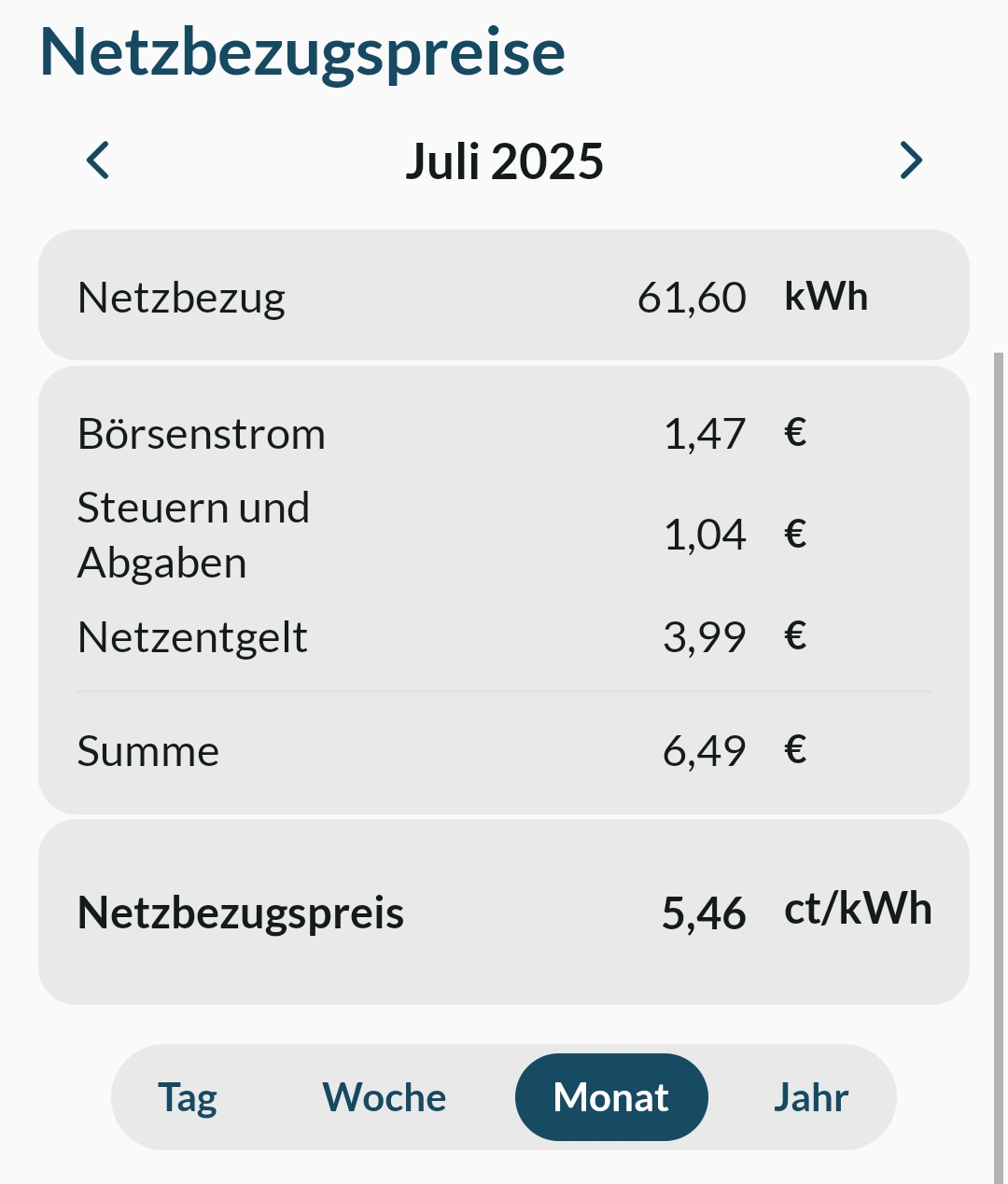
The Final Product

Here you can see a Screenshot how it looks in App.

Closing Thoughts

I hope you enjoyed reading this as much as I enjoyed putting it together. Hopefully, you found it interesting and took away something new for your first ETL-Pipeline.

A big thank you to my awesome colleagues Robert and Becky for the great preparation!

I was lucky to pick it up in a greate state and only had to add final touches.

Thanks for reading!

Geri is a Senior Cloud Consultant at superluminar.
He is passionate about clean code, well architected applications and new technologies.

You can follow on Geri on LinkedIn.
Or follow his cats on Instagram.